Volume rendering, a new feature in Mathematica 9, provides an efficient way to visualize very large data sets. I first learned of this feature from reading Jeffery Bryant’s post on the Wolfram blog. Bryant’s post dealt with simulating galatical collisions. Galaxies have hundreds of billions of stars, so visualizing them as dynamically interacting clouds of points is computationally difficult. Volume rendering provides a solution.

In today’s post, we will use volume rendering for a more prosaic example: color analysis of a photo of puppies.

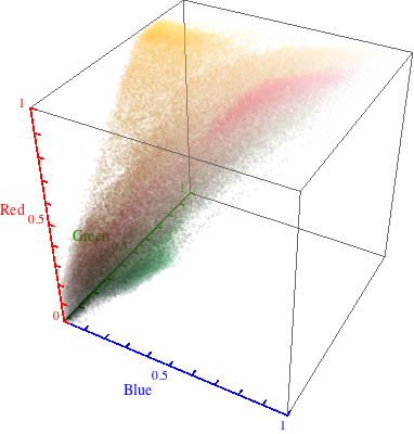
This image contains 589,824 pixels, each of is represented by a three-dimensional vector corresponding to its RGB color (the levels of red, green, and blue for the pixel). We can plot the pixels as points in three-dimensional color space. This is similar to what we did in a previous post about stolen art. Our picture is not huge, so plotting points would work. With very large data sets, though, plotting individual points becomes unmanageable (particularly when the position and properties of the points change in time). An image created with volume rendering is less computationally intensive.

Volume rendering is a broad term for a variety of techniques used to display three-dimensional data on a screen. Many of these techniques are built into Mathematica’s core visualization functions, like Image3D and Raster3D. Before we can make use of these built-in capabilities, we need to process our data.

The space is divided into tiny grid cells, and the number of points in each grid cell is counted. In Mathematica, this can be accomplished with BinCounts. These numbers are used to assign an opacity to each grid cell. The data is represented by a three-dimensional array, where each entry is a four-dimensional vector. The first three entries of the each four-dimensional vector represent the RGB color levels; the fourth is the opacity. This array of data can be displayed using Raster3D.

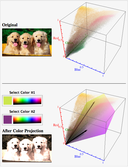
This more efficient way of displaying data is helpful for creating interactive content. In the example below (download CDF), the original puppy image is shown, along with its pixels plotted in color space. Below the original, you can select two colors by clicking on different locations in the color spectrum bars. The two colors you choose form a basis for a plane in RGB colorspace, and this is displayed to the right. The pixels in the puppy image have their colors projected on to the plane spanned by these selected colors. The resulting puppy image is shown. Essentially, you are looking at what the picture would look like if your color palette was limited to a two-dimensional color space instead of a three-dimensional one. You can drag the color space images to change perspective.

If you have a very large (millions of points) data set in three dimensions, consider using tools like Raster3D and Image3D instead of simply plotting all the points!