As a general rule, you should not transform your data to try to fit a linear model. But proportions can be tricky. If the proportion data do not arise from a binomial process (e.g., proportion of a leaf consumed by a caterpillar), then transformation is still the best option. In an excellent paper, David Warton and Francis Hui propose that the conventional transformation for proportion data (i.e., arcsine square root) is asinine, particularly if you have binomial data, and that the logit transformation is preferable for non-binomial proportion data.

The objective of this post is simply to demonstrate how to transform the axes of plots in R, but the context of the example is the logit transformation of non-binomial proportion data. First, we need to generate some data.

reps = 5
sim.data = data.frame(Trt=c(rep("A",reps), rep("B",reps), rep("C",reps)), 
                      Response = c(runif(reps,0,0.4), runif(reps,0.3,0.7), runif(reps,0.6,1)))
eps = min(sim.data$Response)
sim.data$Trans = log((sim.data$Response+eps)/(1-sim.data$Response+eps))

The logit transformation is -Inf at 0 and Inf at 1, but adding a small amount (eps in code above) to both the numerator and denominator of the transformation solves that problem.

Next we run a simple linear model and calculate the predicted means and confidence intervals.

model = lm(Trans~Trt,sim.data)
nd = expand.grid(Trt=unique(sim.data$Trt))
results = data.frame(nd,predict(model,newdata=nd,interval="confidence"))

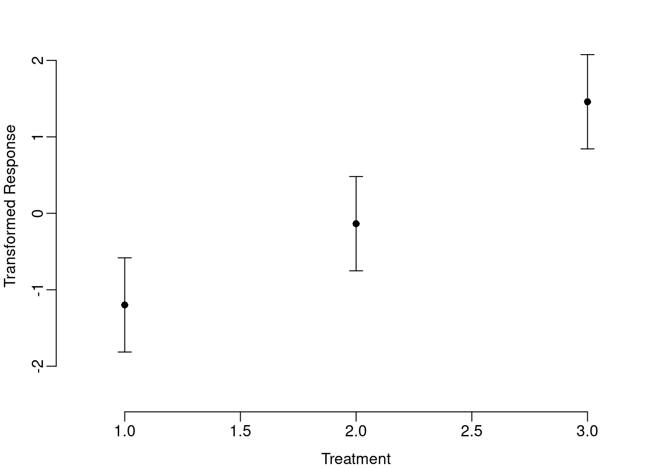
The plotrix package includes a function for easily plotting points with error bars. The code below produces a figure with the transformed response variable.

library(plotrix)
par(mai=c(0.6,0.6,0,0), mgp=c(2,0.5,0))
with(results, 
     plotCI(1:3, fit, li=lwr, ui=upr, pch=16, xlim=c(0.8,3.2), 
            ylim=c(min(sim.data$Trans), max(sim.data$Trans)), bty="n", 
            xlab="Treatment", ylab="Transformed Response"))

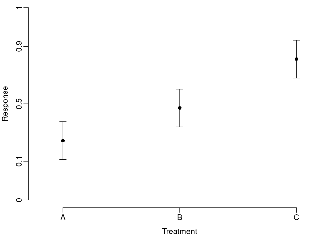
The transformed axis allows the reader to infer treatment effects, but is not easily interpreted. Also, the plotCI function is based on a scatter plot and requires numeric input for both x- and y-variables. But both the transformed y-axis and the mislabeled x-axis are easily changed. The general approach is to tell R to exclude one or both of the axes when drawing the plot and then use the axis function to customize the axes by telling R which labels to use and where to put them. In the case of the transformed y-axis, we want labels that range from 0 to 1 and we will put those labels at the value of the corresponding logit transformation.

y.labels = c(0,0.1,0.5,0.9,1)
y.at = log((y.labels+eps)/(1-y.labels+eps))

We exclude the axes from the plot with the argument axes=F and add our custom axes at the bottom, axis(1), and left, axis(2), of the plot.

par(mai=c(0.6,0.6,0,0), mgp=c(2,0.5,0))
with(results, 
     plotCI(1:3, fit, li=lwr, ui=upr, pch=16, xlim=c(0.8,3.2), 
            ylim=c(head(y.at,1), tail(y.at,1)), bty="n", 
            xlab="Treatment", ylab="Response", axes=F))
axis(1, labels=c("A","B","C"), at=1:3)
axis(2, labels=y.labels, at=y.at)

The back-transformed axis reveals a few key properties of the transformation (i.e., symmetry around 0.5, compressed scale in the middle of the distribution, and spread scale at the ends of the distribution), but obscures the fact that the confidence intervals are not symmetric around the mean.

Alternatively, you can back transform the predicted values from the linear model.

results$orig.fit = (((1/eps)+1)*exp(results$fit)-1)/((1/eps)*exp(results$fit)+(1/eps))
results$orig.lwr = (((1/eps)+1)*exp(results$lwr)-1)/((1/eps)*exp(results$lwr)+(1/eps))
results$orig.upr = (((1/eps)+1)*exp(results$upr)-1)/((1/eps)*exp(results$upr)+(1/eps))

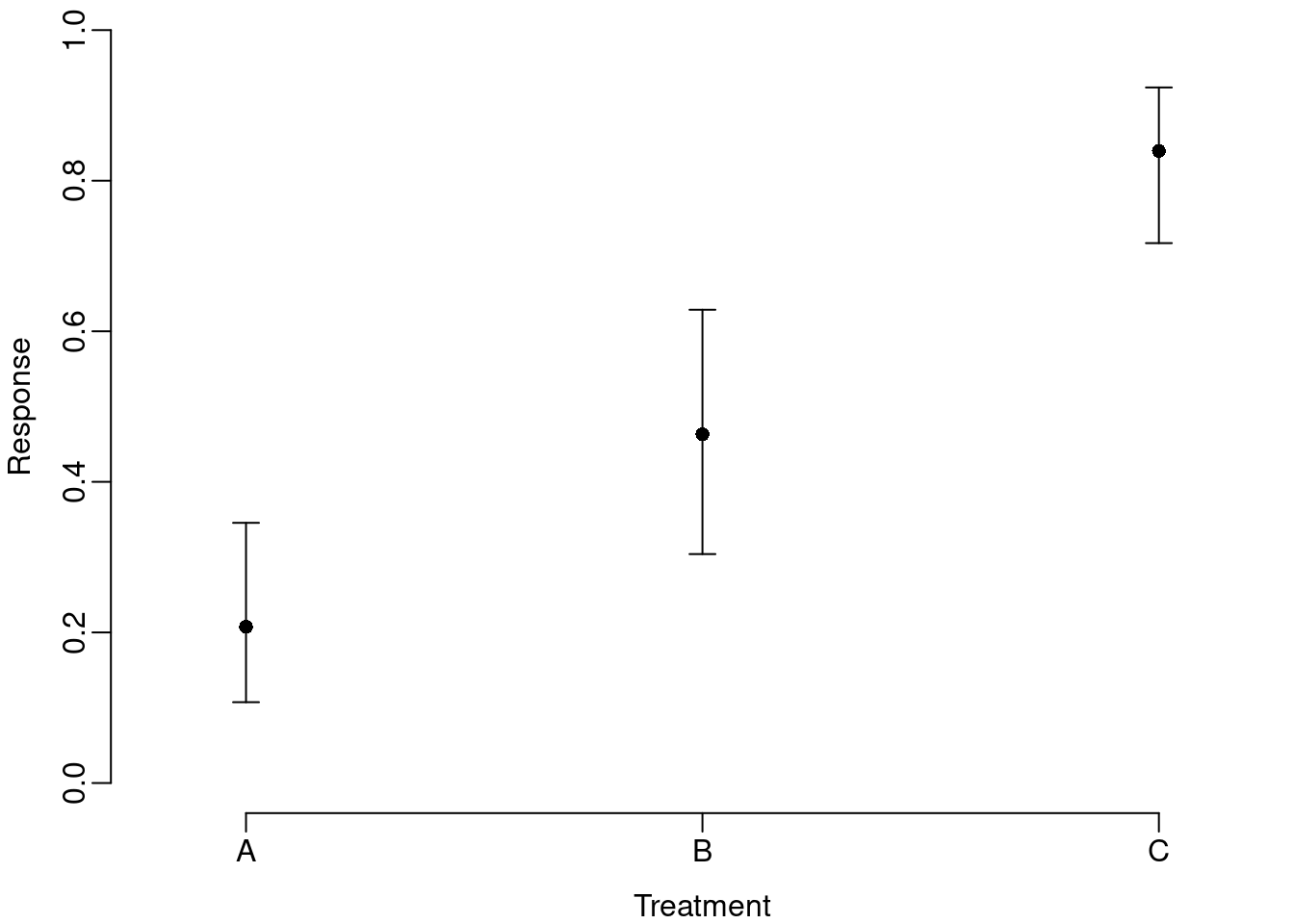
And plot them on the original scale.

par(mai=c(0.6,0.6,0,0), mgp=c(2,0.5,0))
with(results, 
     plotCI(1:3, orig.fit, li=orig.lwr, ui=orig.upr, pch=16, 
            xlim=c(0.8,3.2), ylim=c(0,1), bty="n", xlab="Treatment", 
            ylab="Response", xaxt="n"))
axis(1, labels=c("A","B","C"), at=1:3)

This version provides the more familiar linear y-axis and illustrates the asymmetry in the confidence intervals, but does not confront the reader with the key properties of the transformation.