Mathematica’s NDSolve command is great for numerically solving ordinary differential equations, differential algebraic equations, and many partial differential equations. Most of the integration details are handled automatically, out of the user’s sight. NDSolve switches between integration schemes based on the problem at hand, adapting step sizes and monitoring stiffness as it goes. Advanced users can override these options, customizing NDSolve to their needs.

Sadly, some types of PDEs are beyond NDSolve’s capabilities. Confronted with one of these PDEs, a user must resort to a more “manual” procedure to find a numerical solution. In this post, we’ll examine a few tricks that can make this process easier.

Consider the following PDE:

We seek a solution, f(x,y) on the domain [0,10]x[0,10]. If you try to enter this elliptic PDE into NDSolve, Mathematica will vigorously protest. Instead, you can try to implement a finite difference method.

First, we will divide the domain into a grid. To keep things simple, we will use 1x1 squares.

xgrid = Range[0, 10];
ygrid = Range[0, 10];
grid = Outer[{#1, #2} &;, xgrid, ygrid];

We next make an array of the (as of yet unknown) values that f takes at each point of the grid.

values = Outer[f[#1, #2] &, xgrid, ygrid];

At each grid point, we will replace the derivatives in our PDE with linear combinations of values at neighboring grid points. If you have ever taken Calculus, this idea should sound very familiar– it is essentially like approximating the slope of a line tangent to a graph with the slope of a secant line.

To determine which linear combination of values to use for the different derivatives at the different grid points, we make use of an obscure Mathematica command:

NDSolve`FiniteDifferenceDerivative

The first argument is the type of derivative (for example {2,0} means the second-order derivative with respect to x). The second argument is the grid. The third argument is the array of (unknown) values.

NDSolve`FiniteDifferenceDerivative[{2, 0}, {xgrid, ygrid}, values];

This returns an array. Each entry in the array is the approximation to desired derivative at a particular grid point. For example, one such entry is:

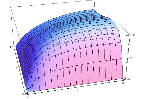
NDSolve`FiniteDifferenceDerivative[{2, 0}, {xgrid, ygrid}, values][[4, 5]]

-(1/12) f[1, 4] + 4/3 f[2, 4] - 5/2 f[3, 4] + 4/3 f[4, 4] - 1/12 f[5, 4]

We can see that the second order derivative with respect to x at the point (3,4) is expressed as a linear combination of values of f. Note that it is at the point (3,4) not (4,5) because the part specifications start at index 1, while the grid coordinates start at zero. With this tool, we can replace the partial differential equation for the unknown function f with a large number of linear algebraic equations for the unknown values f(i,j). It is necessary to replace some of these equations with appropriate boundary conditions (in our example, two of the boundaries are absorbing, and two are reflecting). Once this is done, we can solve for all of the f(i,j) values. I’ll spare you the code¹, and just show the resulting picture of the approximation to the solution:

In conclusion, we can see that, even when NDSolve can’t handle a PDE, Mathematica has some hidden gems that can make life easier!