Numerical Integration

One of the first topics in any introductory differential equations course is Euler’s method, an algorithm for numerically solving an ordinary differential equation. In this method, time is discretized into small steps, and the value of the solution at each step is approximated using the slope of the tangent line. The approximation gets better when the time domain is partitioned into more, smaller steps.

There is also an Euler’s method (usually called the Euler-Maruyama method) for integrating stochastic differential equations. Beyond the first week of a differential equations course, nobody actually uses Euler’s method to solve DE’s. Almost immediately, Euler’s method is discarded in favor of more sophisticated and efficient algorithms.

In the realm of stochastic differential equations, there are much more efficient methods than the Euler-Maruyama method. While most modelers would think it ridiculous to use Euler’s method in the deterministic setting, they are hesitant to move beyond the Euler-Maruyama method in the stochastic setting.

Before proceeding, let’s discuss how to measure the efficiencies of stochastic differential equation numerical integration schemes. Of course, the accuracy of a given method depends on the step-size that is used. The nature of this dependence is important: the accuracy of some methods will increase faster with decreasing step-size than the accuracy of other methods will. In essence, some methods give you more bang for your buck when decreasing step-size.

The strong and the weak

We can measure the accuracy of a stochastic numerical scheme in two ways: the strong sense and the weak sense. You can read about the mathematical distinction between these two concepts in any stochastic processes text, but I’ll try to give you an intuitive analogy here.

Suppose that you are trying to simulate the path of a fly as it meanders around your Labor Day picnic. If you are given all of the information about the different random events that influence the fly (wind gusts, etc.) you should be able to simulate the fly’s trajectory very closely. You will be off by a little, because the fly’s trajectory is a continuous process, and your simulation scheme has discrete chunks of time. Now, measure how far the simulated trajectory’s endpoint was from the endpoint of the fly’s actual trajectory. Do the same thing for many, many different sets of random events that affect the fly. If your simulation does well on average, then it is accurate in the strong sense.

Alternatively, you might be interested, not in tracing the path of any particular fly, but rather in just knowing the broad statistical properties of the position of a swarm of flies. If the position of your simulated swarm of flies has close to the same mean, variance, etc. of the actual swarm of flies, your simulation has done well in the weak sense.

Milstein’s method

Today, we are going to examine Milstein’s method for numerically solving SDEs. The subtle distinction between strong and weak approximation is important. In the weak sense, the Euler-Maruyama method and Milstein’s method behave similarly (both are of order one). In the strong sense, though, Milstein’s method is much more accurate (it is of order one, while the Euler-Maruyama method is of order 1/2).

Consider the following stochastic differential equation (in vector form):

In component form, this can be written as:

The Euler-Maruyama method for this SDE can be written in vector form as:

Or in component form as:

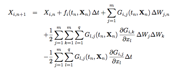
The Milstein method can be written in component form as:

If the noise sources are commutative, this simplifies to:

We can code each of these methods as follows: First, for each method, define the time step, the appropriate vector of functions f[{x1,x2}] and matrix of functions g[{x1,x2}].

euler[{x1_, x2_}] :=
Module[{dW1, dW2}, dW1 = RandomVariate[NormalDistribution[0, (dt)^(1/2)]];
dW2 = RandomVariate[NormalDistribution[0, (dt)^(1/2)]]; {x1, x2} +
f[{x1, x2}]*dt + {g[{x1, x2}][[1, 1]]*dW1, g[{x1, x2}][[2, 2]]*dW2}]

Next, for each method, create a function that maps a given point {x1, x2} of the trajectory to its position after the next time step:

milstein[{x1_, x2_}] :=
Module[{dW1, dW2}, dW1 = RandomVariate[NormalDistribution[0, (dt)^(1/2)]];
dW2 = RandomVariate[NormalDistribution[0, (dt)^(1/2)]]; {x1, x2} +
f[{x1, x2}]*dt + {g[{x1, x2}][[1, 1]]*dW1,
g[{x1, x2}][[2, 2]]*dW2} + (1/
2) ({g[{x1, x2}][[1,
1]]*(D[g[{u, v}][[1, 1]], u] /. {u ->x1, v-> x2})*dW1*dW1 +
g[{x1, x2}][[2,
2]]*(D[g[{u, v}][[1, 1]], v] /. {u ->x1, v -> x2})*dW2*dW1,
g[{x1, x2}][[1,
1]]*(D[g[{u, v}][[2, 2]], u] /. {u -> x1, v -> x2})*dW1*dW2 +
g[{x1, x2}][[2,
2]]*(D[g[{u, v}][[2, 2]], v] /. {u -> x1, v -> x2})*dW2*dW2}) - (1/
2)*(dt)*({g[{x1, x2}][[1, 1]]*D[g[{u, v}][[1, 1]], u] /. {u -> x1,
v -> x2},
g[{x1, x2}][[2, 2]]*D[g[{u, v}][[2, 2]], v] /. {u -> x1, v ->x2}})]

Now use Mathematica’s NestList command to generate a full trajectory:

ListPlot[NestList[milstein[#]&;, {900, 400}, 100000], Joined -> True,
PlotRange-> {{0, 2500}, {0, 1500}}, AspectRatio -> 1]

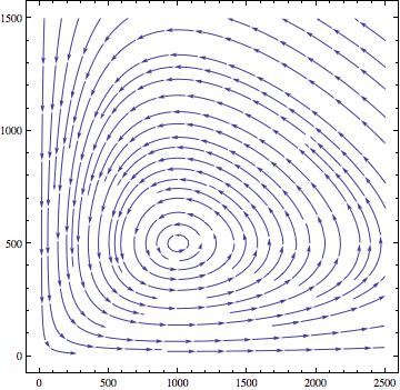
We can demonstrate this with a Lotka-Volterra model that includes demographic stochasticity. Here is the vector plot of the underlying deterministic skeleton:

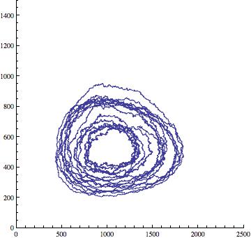
And here is a sample trajectory obtained using Milstein’s method:

Happy Labor Day! Now back to work :(