Comparing stolen paintings: Picasso and Matisse
Art Heist
Last week, burglars stole seven paintings from the Kunsthal museum in Rotterdam. The paintings included works by Picasso, Monet, Gauguin, and Matisse. The loot is likely worth hundreds of millions of dollars, but the loss of these great pieces surpasses anything that can be calculated as a monetary figure. Art is unquantifiable, right? Yes, but it is still fun to do data analysis on paintings. In today’s post, we will explore how Mathematica’s image processing capabilities can be used to compare two of the paintings stolen from the Kunsthal.
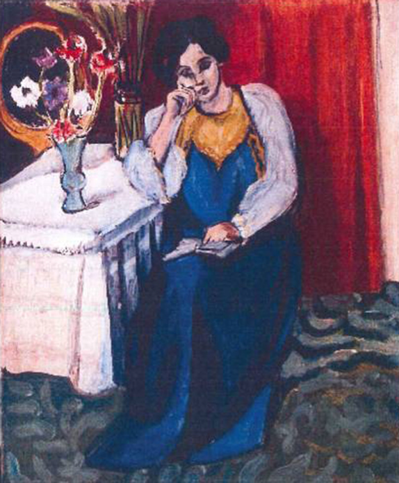
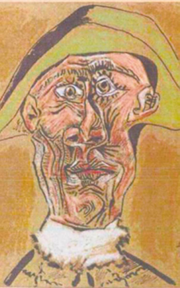
Let’s consider Matisse’s “Reading Girl in White and Yellow” (1919) and Picasso’s “Harlequin Head” (1971).
Matisse
Picasso
Color space
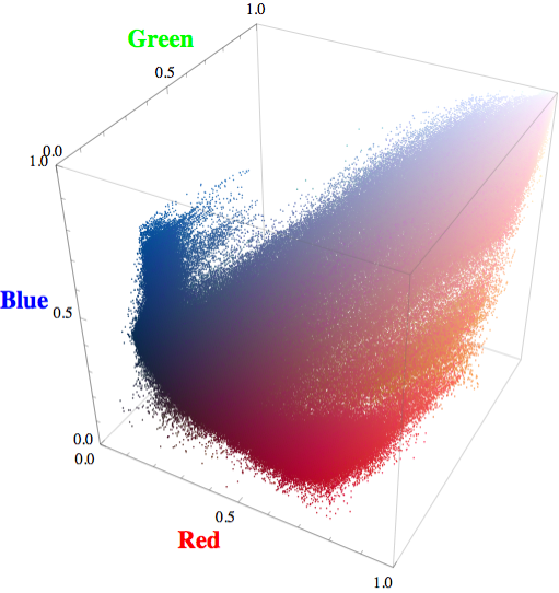
Mathematica represents each pixel with a vector whose entries correspond to the relative intensity of red, green, and blue channels, respectively. We can plot each pixel of the painting as a point in three-dimensional color space.
Matisse
Picasso
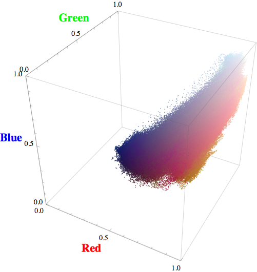
You can see that the Matisse draws from a larger color palette, and hence the points span a broader area of the color space.
Entropy
Entropy provides a way to measure the information contained in a painting. A full explanation of this topic is beyond the scope of this blog, but a few general concepts are worth noting. When dealing with a distribution of different colors of pixels, the concepts of information, uncertainty, and evenness are roughly equivalent.
Suppose that you have a totally random painting, so that the pixels are evenly distributed across the color spectrum. Further suppose that you have the ability to reach into the painting and pull out a pixel at random. Don’t look at the pixel. Just hold it in your hand. Clearly, you are very uncertain about the color of the pixel that lies in your palm. Now open your hand and look at the pixel. You had almost no idea what color the pixel would be; now you know. The act of observing that pixel conveys a large amount of information to you.
Conversely, suppose that you have a painting in which 95% of pixels are pure blue. If you pick a pixel at random, then, even before you open your hand to look at it, you are pretty certain about what color you are holding. Looking at the pixel probably will not convey much information to you (seeing that it is blue be terribly surprising). This is why high uncertainty means high information (high entropy), and low uncertainty means low information (low entropy).
Things get more complicated when we consider the spatial structure of pixels in a picture. For example, if you were to reach into Matisse’s painting and take a pixel from a spot on the tablecloth, you’d be relatively certain about obtaining a white pixel. If you take a pixel from the region around the flowers, though, you have higher uncertainty about its color. Entropy takes different values in different locations.
Entropy and spatial scale
We’d like to assign an entropy value to every point in a painting; this will allow us to see which areas of the painting are high entropy, and which are low. To define the entropy at a point, we take a small neighborhood of pixels around that point, and calculate the entropy of this collection of pixels. The size of the neighborhood matters: in general, we will use a 2r+1 x 2r+1 square, and will adjust r to examine different scales.
Here is what the entropy of the Matisse painting looks like for r=1 (black is low entropy, white is high).
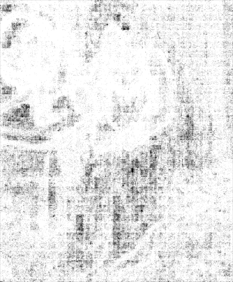
Matisse, r=20:
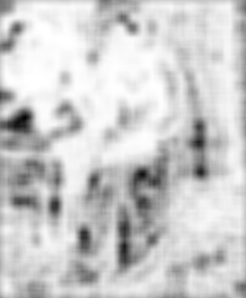
Picasso, r=1:
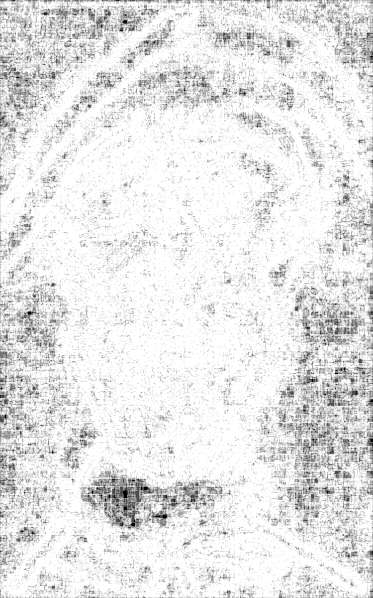
And for r=20:
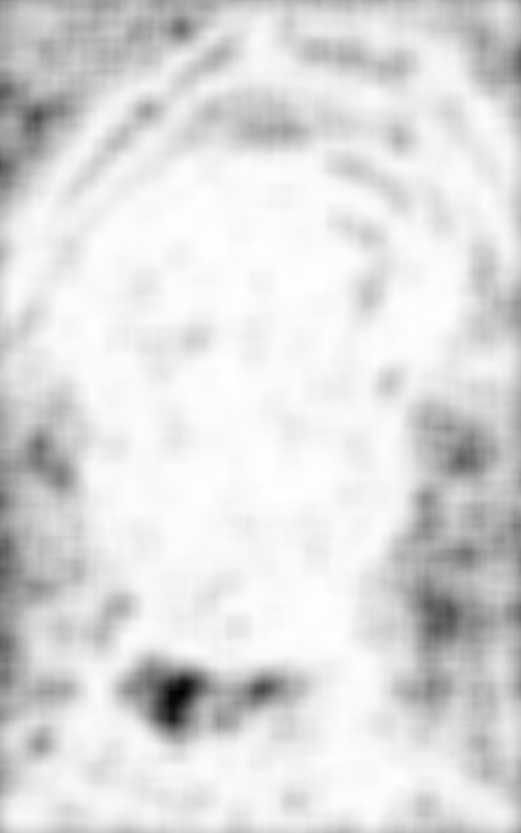
Mean Entropy per pixel
Let’s compare the information per pixel in the two paintings. Below is a plot of how the difference between the paintings’ average entropy per pixel (Matisse average entropy per pixel minus Picasso average entropy per pixel) changes with neighborhood size. Negative values indicate that the Picasso painting has higher entropy per pixel at that scale; positive values indicate that the Matisse painting does.
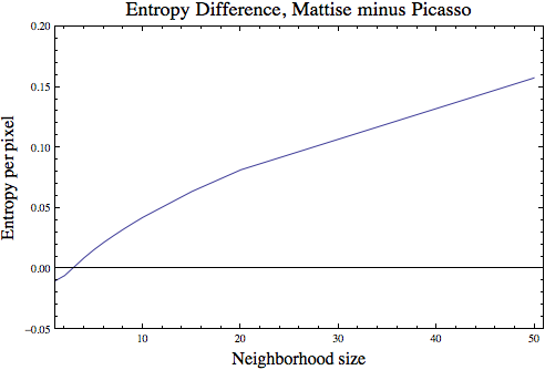
Interestingly, at very small scales the Picasso painting has higher entropy, while at larger scales the Matisse does. At very small scales, there is more structural complexity and heterogeneity in the Picasso than the Matisse. At larger scales, we see that the Matisse draws from a broader spectrum of color, and thus contains a wider distribution of pixel types.
In the calculations above, each pixel color is classified as distinct. With 3 color channels, and 256 possible values for each channel, this means that there are over 16 million possible distinct colors. In some situation, this fine distinction between colors might be more than we want to consider (see code below).
Final thought
If the thieves damage the paintings, let’s hope they damage the low entropy regions identified above. It will be easier to reconstruct those regions from surrounding pixels than the regions that have higher information content.
Code
First, import the data:
matisse = ImageData[Import["file"]];
 picasso = ImageData[Import["file"]];
This calculates the neighbor pixels in a 2r+1 x 2r+1 block around a pixel at location (i,j) in picture “data”:
neighbors[data_, {i_, j_}, r_] :=
 Flatten[Take[
  data, {Clip[i - r, {1, Dimensions[data][[1]]}],
   Clip[i + r, {1, Dimensions[data][[1]]}]}, {Clip[
   j - r, {1, Dimensions[data][[2]]}],
   Clip[j + r, {1, Dimensions[data][[2]]}]}], 1]
This calculates the entropy of a pixel at position (i,j) in painting “data” using neighborhood size r:
localEntropy[data_, {i_, j_}, r_] := Entropy[neighbors[data, {i, j}, r]] // NThis maps that entropy to each pixel:
entropyFilter[data_, r_] := MapIndexed[localEntropy[data, #2, r]&;, data, {2}]This calculates the average entropy per pixel:
meanEntropy[data_, r_] :=
 Total[Flatten[entropyFilter[data, r], 1]]/(Dimensions[data][[2]]*
   Dimensions[data][[1]])
Alternatively, Mathematica has an EntropyFilter function that can be applied directly, but this does not offer the ability for a customization for different color discretizations.
To handle a “coarser” view of color (that is, to treat very similar colors as the same), can use the SameTest option within Mathematica’s Entropy function. Simply replace the localEntropy function defined above with this smoothLocalEntropy function:
smoothLocalEntropy[data_, {i_, j_}, r_] :=
N[Entropy[Flatten[neighbors[data, {i, j}, r], 1],
SameTest-> (Norm[#1 - #2]< 10^-2)&]]