In today’s blog post, we’ll show you how to use Mathematica’s plotting features to visualize geospatial data.

Baintha Brakk, aka The Ogre, is a mountain in the Karakoram range in northern Pakistan. It is “only” the 87th highest mountain on the planet (23,901 feet), but it’s among the technically most difficult to climb.

Chris Bonington and Doug Scott made the first ascent in 1977. Early in the descent, Scott broke both his legs in a repelling accident. The ensuing struggle to get down alive was epic.

The Ogre was not climbed again until 2001 (although there were many unsuccessful attempts in the intervening years). To my knowledge, the 1977 and 2001 expeditions are still the only successful ones.

Note: For another intense account of high altitude survival, check out the most recent episode of Family Guy, Into Fat Air.

The USGS’s Earth Explorer is a great resource for finding and downloading digital elevation data. Mathematica can import a variety of geospatial data formats. In the following example, I’ve used the GeoTIFF format.

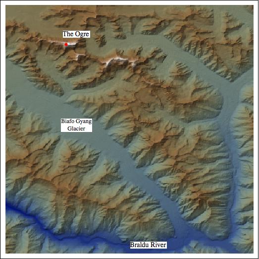
In Mathematica, an array of elevation data can be conveniently displayed with the ReliefPlot function.

We can fit an interpolating polynomial to the data using Mathematica’s Interpolation function. This is useful, because it represents the terrain as a smooth function, so gradients can be calculated.

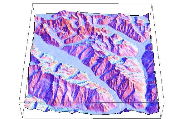
Here is what a plot of a (very high order) interpolating polynomial fit to the data looks like:

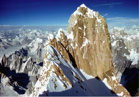
Of course, polynomials can never quite capture the real deal (photo credit: Doug Scott):