You’ve probably heard of the traveling salesman problem: given a set of cities, what is the shortest possible route that visits each city exactly once and returns to the origin city? This problem pops up in a huge number of applications.

For the purposes of this post, let’s focus on a concrete example: a musician is planning a tour and wants to travel as efficiently as possible. Suppose that concerts are to be held in the following cities (with an encore concert in the origin city): Anchorage, Athens, Barrow, Berlin, Brussels, Cairo, Copenhagen, Denver, Detroit, Dublin, Helsinki, Istanbul, Jerusalem, Kabul, Lagos, Lisbon, London, Los Angeles, Miami, Moscow, Murmansk, New York, Prague, Reykjavik, Rome, Seattle, Stockholm, and Toronto.

Perhaps you’ll object that this is an unlikely list, because it includes several high latitude cities with limited concert venues. Musicians can get sent to some pretty obscure locations, though. Take the rapper Pitbull’s recent trip to Kodiak, for example. Bear with me.

Fortunately, Mathematica has a built-in function, FindShortestTour to help compute the solution to our problem. Before we get too excited, though, we should remember that the world is not flat, and hence we won’t be able to use our usual Euclidean distance metric.

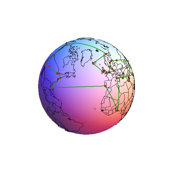
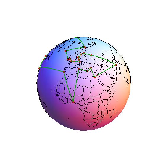
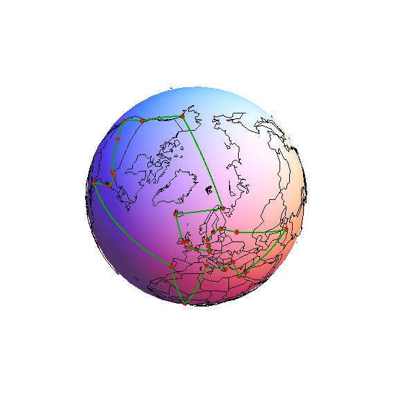
I’ll walk you through some code that computes and displays the solution to our hypothetical problem. Most of this code is adapted from an example in Mathematica’s documentation. For those who want the end picture with no code, here you go:

Now, let’s turn to the code. First, we can make use of Wolfram’s extensive databases, and find the latitudinal and longitudinal coordinates of all of our cities.

cities={"Barrow","Anchorage","Lagos","Murmansk","Reykjavik","Helsinki","Stockholm","Copenhagen","London","NewYork","Kabul","Berlin","Rome","Seattle","Denver","Detroit","Brussels","Lisbon","Dublin","Moscow","Los Angeles","Toronto","Miami","Cairo","Prague","Jerusalem","Istanbul","Athens"};
citylocations=CityData\[#,"Coordinates"\]&/@cities;

Next, we want to be able to convert things from latitude and longitude to Cartesian coordinates 3-space. We will work in units of kilometers. The position function below accomplishes this:

earthRad = 6378.7;
positionVec[{u_, v_}] := {Cos[v °] Cos[u °], Sin[v °] Cos[u °], 
                          Sin[u °]};
position[{u_,v_}] := earthRad*positionVec[{u,v}]

The length of an arc between two points with specified latitudinal and longitudinal coordinates can be computed using the distance function defined below. Note the use of Mathematica’s built-in function VectorAngle.

distance[{u1_,v1_},{u2_,v2_}] := earthRad * VectorAngle[
                       positionVec[{u1,v1}], positionVec[{u2,v2}]];

The built-in FindShortestTour command can accommodate our distance metric. We define “tour” to be the list Mathematica returns. The first element of this list is the total distance of the journey; the second is the list of indices corresponding to the cities, and it specifies the order in which they are to be visited.

tour=FindShortestTour[citylocations, DistanceFunction->distance]
{47565.1,{1,9,17,25,12,8,7,6,20,11,26,24,27,28,13,3,18,23,10,22,16,15,21,14,2,4,5,19}}

Now we get to the interesting part–displaying our results.

First, we’d like a function to connect a given pair of cities with a nice arc. The most important feature of this chunk of code is the use of RotationTransform. This built-in function takes three arguments. The first is an angle, the second is a pair of vectors. The pair of vectors in the second argument specify the plane in which the rotation will occur. RotationTransform outputs a function (a rotation matrix) that can be applied to a point.

I use NestList (as you will see, this is one of the Mathematica functions I use the most) to iteratively perform rotation transforms, outputting a sequence of positions on the surface of the sphere between the two cities.

makearc[{u1_,v1_},{u2_,v2_}\]:=
Module[ {city1=position[{u1,v1}], city2=position[{u2,v2}], dist},
dist=VectorAngle[city1,city2];
NestList[(Evaluate[
   RotationTransform[dist/Ceiling[100*dist],{city1, city2}][#]])&, 
                                       city1, Ceiling[100*dist]]]

Next, we’d like to make nice arcs between each pair of consecutively cities. To get pairs of consecutively visited cities, we use the Partition function. Then we apply our makearc function (defined above) onto the result.

routePic=Apply[makearc,
                  Partition[citylocations[[tour[[2]]]],2,1],{1}];

When we display everything, we want a sphere, a map of the countries of the world, dots for cities, and the path taken by our tour. The latter two things we have all but done, and the first is trivial. Now we just need a map of the countries. To do this, we again use Mathematica’s databases:

countries = CountryData["Countries"];

Each country has an associated schematic polygon, with vertices specified by longitude and latitude. We need to translate that into Cartesian 3-space, and then draw lines connecting these vertices. This can be accomplished with the following command:

Map[Line[Map[position,
         CountryData[#,"SchematicCoordinates"],{-2}]]&, countries]

Finally, putting everything together into a single graphics display:

Graphics3D\[{Sphere\[{0, 0, 0}, 0.99\*earthRad \], 
     Map\[Line\[Map\[position, CountryData\[#, "SchematicCoordinates"\], {-2}\]\] &, countries\],
     {Darker\[Green\], Thick, Line\[routePic\]},
     {Red, PointSize\[Large\],
     Map\[Tooltip\[Point\[position\[CityData\[#, "Coordinates"\]\]\], #\] &, cities\]}}, 
        Boxed -> False, SphericalRegion -> True\]

In Mathematica, it is easy to grab and spin the globe for whatever perspective you want: